Compressible flow is a branch of fluid mechanics that deals with flows having significant changes in fluid density
"Significant changes in fluid density"
- what does that mean?
- propagation of acoustics waves
- high-speed flows
- flows with large pressure variations

- Related to the mean molecular velocity
- Changes with temperature \(\left(c=\sqrt{\gamma R T}\right)\)
- Inversely proportional to the fluid compressibility
- Finite Volume
- structured Meshes
- parallel (MPI/PETSc/SLEPc)
- Time-Marching technique
- explicit three-stage second-order Runge-Kutta
- dual time stepping/residual smoothing/low-speed preconditioning
- Convective fluxes
- third-order low-dissipation upwind scheme
- cube with the side \(L=1.0\ m\)
- resolve acoustic waves in the range \(f=50\ Hz\ -\ 10000\ Hz\)
- 20 cells per wavelength
Upper frequency limit \(\left(f=10000\ Hz\right)\):
\(\lambda=c/f=0.034\ m\ \Rightarrow \Delta x < \lambda/20 = 0.0017\ m\)
Number of cells: \((L/\Delta x)^3>{\class{MyRed}{200 \times 10^6}}\)
- acoustic waves in large domains
- thin boundary layers
- large velocity gradients
- shocks
- high relative velocities (turbomachinery)
- weak acoustic waves in high-energy flows
- acoustic reflections
- back flow
- extrapolation errors
FLOW-INDUCED SOUND
- Shear flows
- Boundary layers
- Combustion
- Turbomachinery blade self noise
- Broadband shock-associated noise

- Numerical accuracy
- Mesh requirements
- Boundary conditions
- Rotor/stator interaction
- Feedback mechanisms
- Buzz-saw noise

- Boundary conditions
- Number of harmonics
- Propagation of acoustics
ACOUSTIC ANALOGIES
The analogy between the non-linear flow and the linear theory of acoustics
Starting point:
continuity equation:
\[\frac{\partial \rho}{\partial t}+\frac{\partial(\rho u_i)}{\partial x_i}=0\]momentum equation:
\[\frac{\partial (\rho u_i)}{\partial t}+\frac{\partial (\rho u_i u_j)}{\partial x_j}=\frac{\partial }{\partial x_j}(\sigma_{ij}-p \delta_{ij})\]Step 1. the temporal derivative of the continuity equation
\[\frac{\partial^2 \rho}{\partial t^2}+{\class{MyRed}{\frac{\partial^2(\rho u_i)}{\partial x_i \partial t}}}=0\]Step 2. the divergence of the momentum equation
\[{\class{MyRed}{\frac{\partial^2 (\rho u_i)}{\partial x_i \partial t}}}+\frac{\partial^2 (\rho u_i u_j)}{\partial x_i \partial x_j}=\frac{\partial^2 }{\partial x_i \partial x_j}(\sigma_{ij}-p \delta_{ij})\]Step 3. eliminate the highlighted terms
\[\frac{\partial^2 \rho}{\partial t^2}=\frac{\partial^2 }{\partial x_i \partial x_j}(\rho u_i u_j - \sigma_{ij} + p \delta_{ij})\]Now, subtracting \({\class{MyBlue}{a_\infty^2\frac{\partial^2 \rho}{\partial x_i^2}}}\) on each side gives us Lighthill's acoustic analogy
\[\frac{\partial^2 \rho}{\partial t^2}-{\class{MyBlue}{a_\infty^2\frac{\partial^2 \rho}{\partial x_i^2}}}=\frac{\partial^2 T_{ij}}{\partial x_i \partial x_j}\]where \(T_{ij}\) is the Lighthill stress tensor defined as
\[T_{ij}=\rho u_i u_j - \sigma_{ij} + (p-{\class{MyBlue}{a_\infty^2\rho}}) \delta_{ij}\](\(a_\infty\) is the speed of sound in an observer location)
| \(\Omega\) | volume containing sound sources |
| \({\mathbf{y}}\) | observer location |
| \({\mathbf{x}}\) | source location |
| \(r\) | distance between source and observer |
| \(\tau_r\) | retarded time |
- A Krylov subspace technique for extraction of global flow field modes
- Post processing technique applied to series of flow field snap shots
- Independent of data origin
- Possible to apply to truncated data sets
Assume linear mapping, \(B\), of the flow dynamics
\[Q^{(n+1)}=BQ^{(n)}\]where \(Q^n\) is the flow field at time \(t^n\) and \(Q^{n+1}\) the flow field at time \(t^{n+1}=(t^n+\Delta t)\)
- \(Q^{(k)},\ k\in\{1, 2, \dots, n+2\}\) is a set of flow-field vectors sampled with a specified frequency
- Differences of consecutive sampled solver states are used to define matrices \(V_n\) and \(V_{n+1}\)
Using SVD, the matrix \(V_n\) can be decomposed as
\[V_n=U\Sigma W^*\]and since \(V_{n+1}=BV_n\)
\[V_{n+1}=BV_n=B U\Sigma W^*\]| \(U\) | \(\left(m\times p\right)\) | \(\Sigma\) | \(\left(p\times p\right)\) | \(W^*\) | \(\left(p\times n\right)\) |
Multiplying both sides by \(U^*\) from the left
\[{\class{MyGreen}{U^*V_{n+1}}}=\underbrace{\class{MyRed}{U^*BU}}_{\class{MyBlue}{C}}{\class{MyGreen}{\Sigma W^*}}\]where \(\class{MyBlue}{C}\) is the projection of the system matrix (\(B\)) on \(U\)
The projected system matrix can now be obtained without direct access to \(\class{MyRed}{B}\) as
\[\class{MyBlue}{C}={\class{MyGreen}{U^*V_{n+1}W\Sigma^{-1}}}\]- \(\class{MyBlue}{C}\) is a \(\left(p\times p\right)\) matrix, \(\left(m \gg n \ge p\right)\)
- The eigenvalues of \(\class{MyBlue}{C}\) gives a good representation of the least damped eigenmodes of \(B\)
- Each eigenmode has a specific frequency
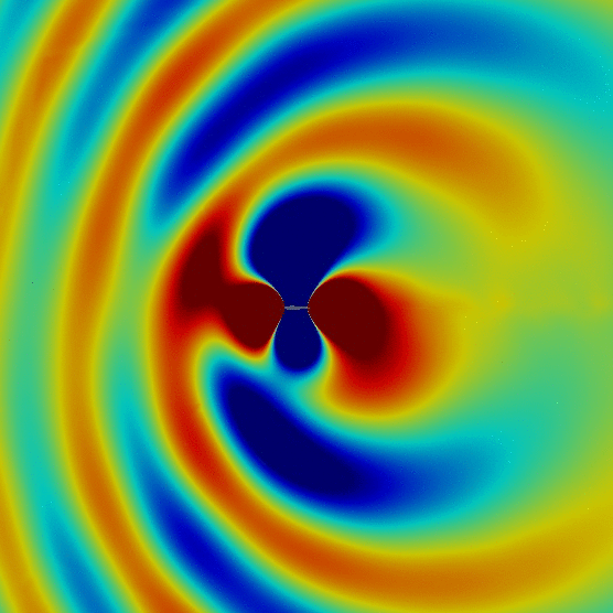

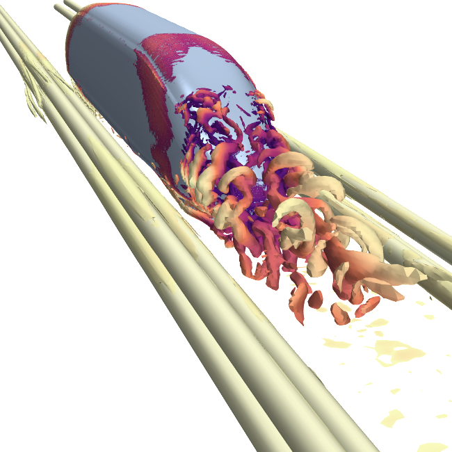
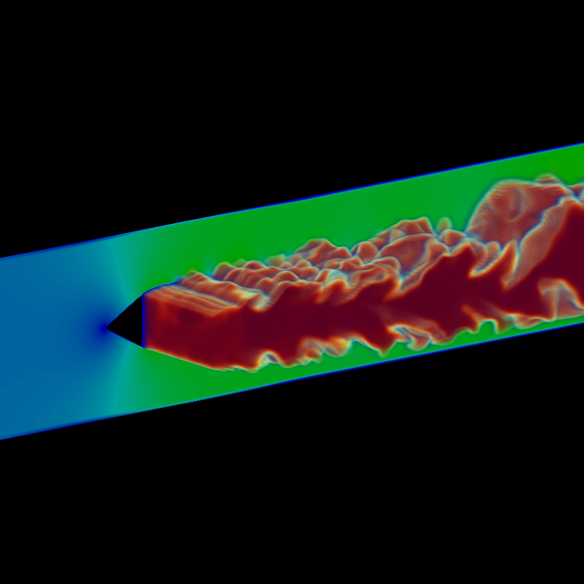
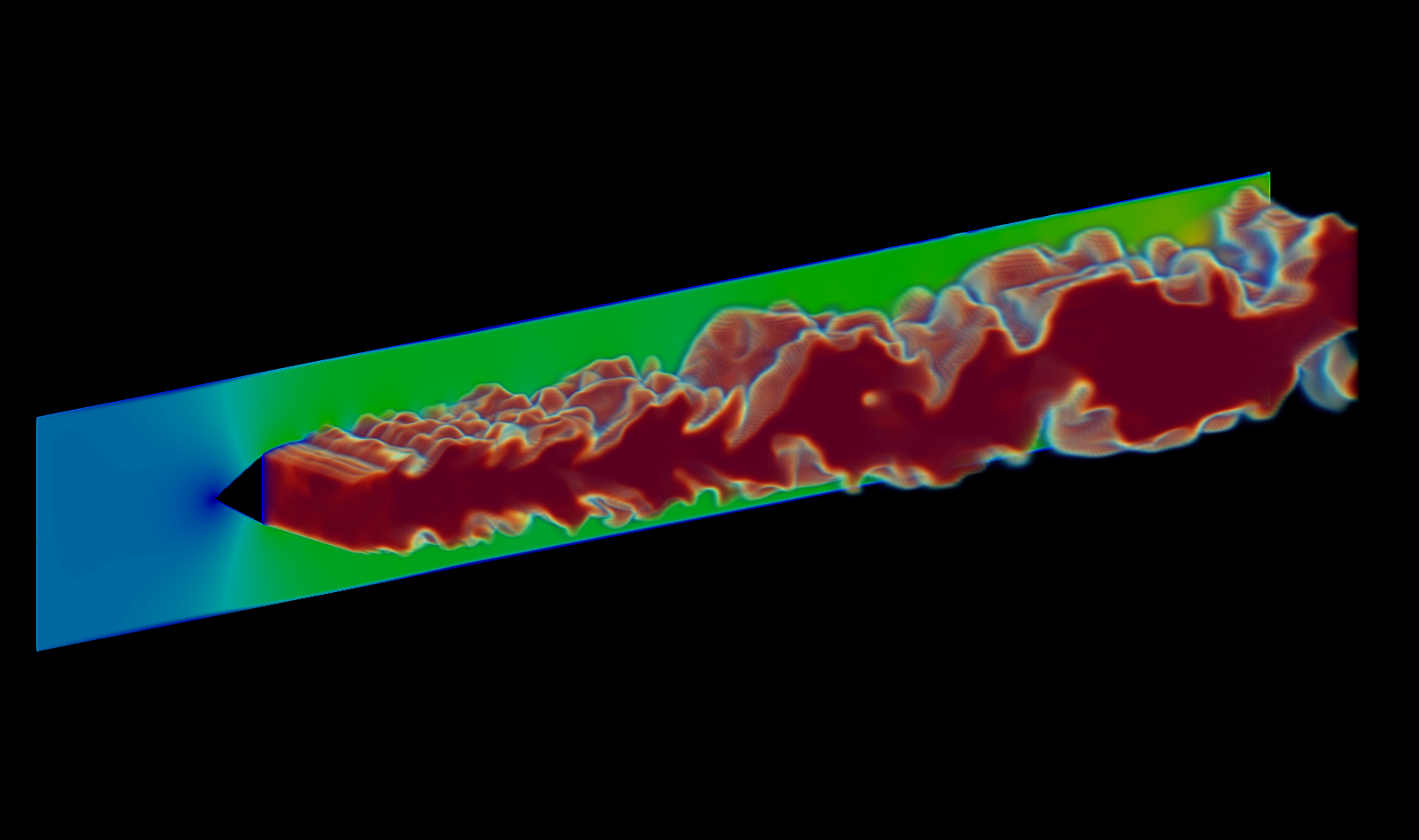
SUPERSONIC JET AOCOUSTICS
Screech tone cancellation using fluid injection


- Compressible LES
- Ffowcs William-Hawking surface integration
- Dynamic Mode Decomposition (DMD)
- Boundary conditions
- Short time step
- Noisy data


- Feedback mechanism:
- flow structures at the nozzle lip
- upstream-traveling disturbances


Helical mode with the screech frequency detected using Dynamic Mode Decomposition (DMD)
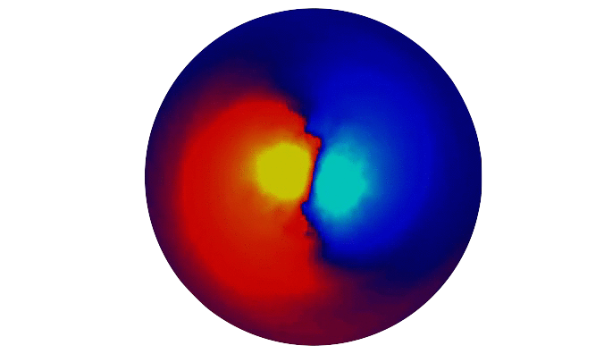
SPACE NOZZLES SIDE LOADS
Prediction of side loads during a space nozzle start-up sequence


- Compressible URANS/DDES
- Dynamic Mode Decomposition
- Short time step
- Noisy data


- Simulated side-loads were lower than measured side-loads but within uncertainty levels
- DMD Identified modes responsible for side-loads and nozzle ovalization
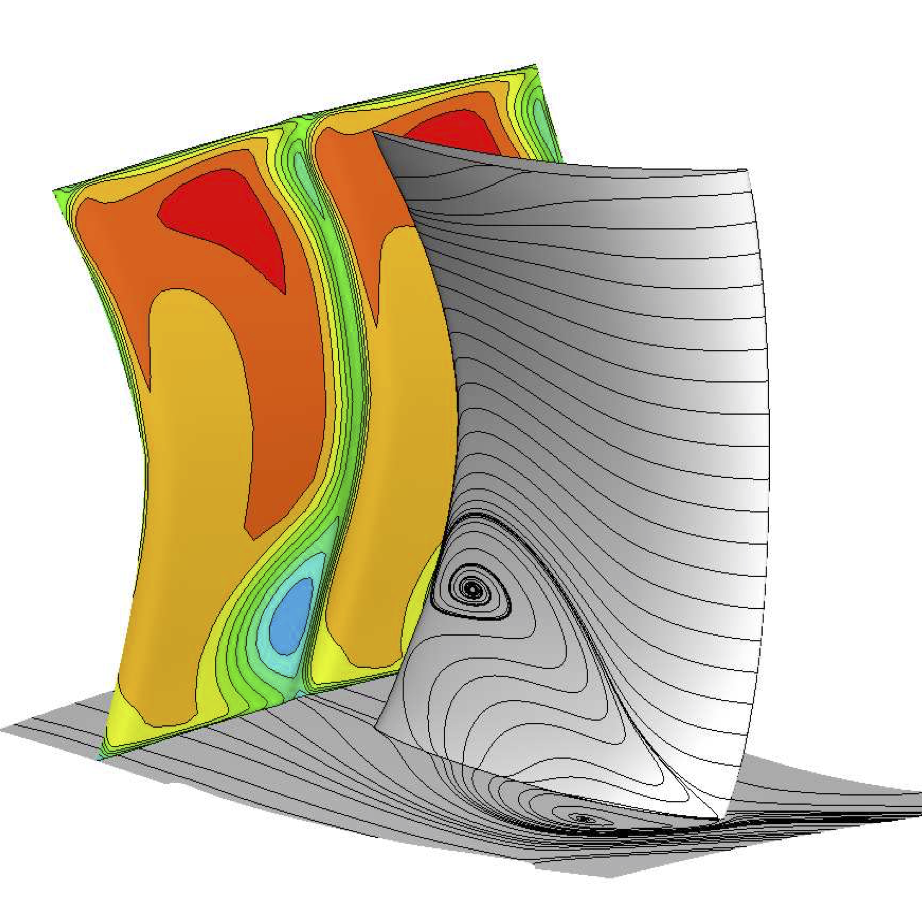
COMPRESSOR DUCT AREODYNAMICS
Investigation of the aerodynamics of an intermediated compressor duct with integrated bleed system


- Compressible DDES
- Spalart-Allmaras
- Short time step
- Bleed tube boundary conditions


- Spalart-Allmaras DDES model implemented
- Significantly improved time-stepping technique
- dual time stepping
- five-stage Runge-Kutta
- implicit residual smoothing
- low-speed preconditioning
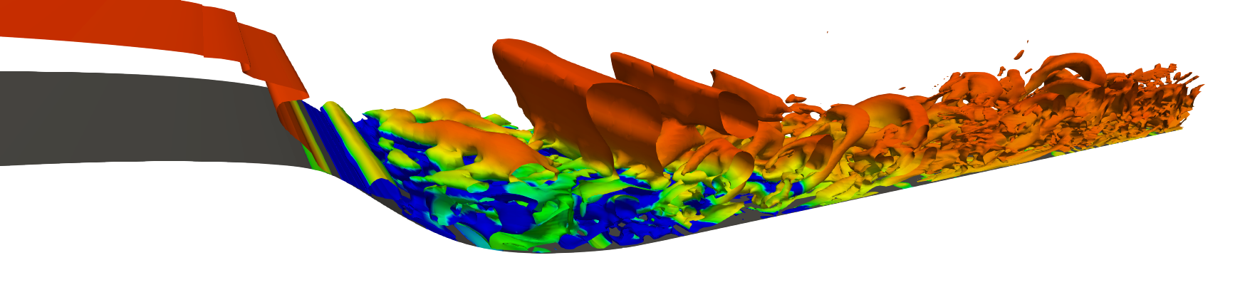
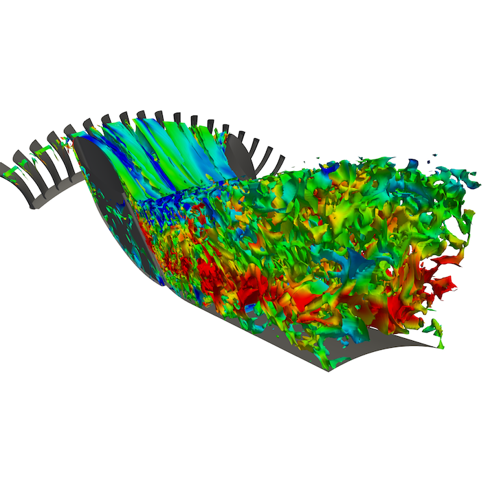
FAN BLADE BROADBAND NOISE GENERATION
Prediction of fan outlet guide vane broadband noise using detailed numerical methods

- Compressible DDES/URANS
- Chorocronic tangential boundaries
- Specified wake-data from upstream rotor
- Inlet synthetic turbulence
- Ffowcs William & Hawking surface integration
- Very short time step
- Tangential boundary feedback loop
- Inlet turbulence

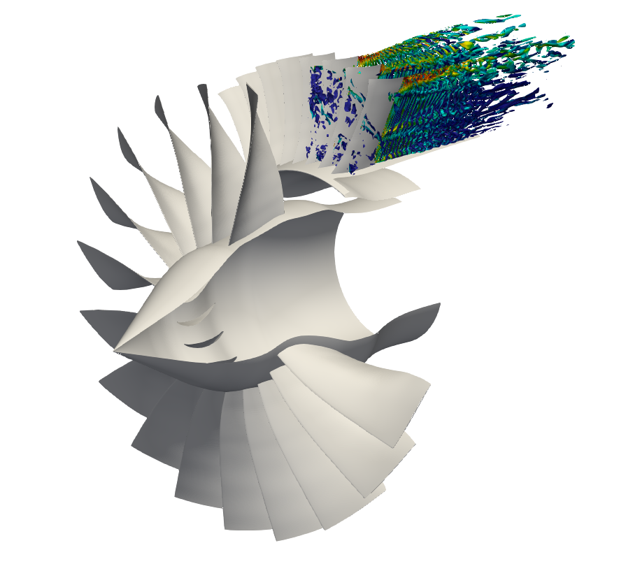
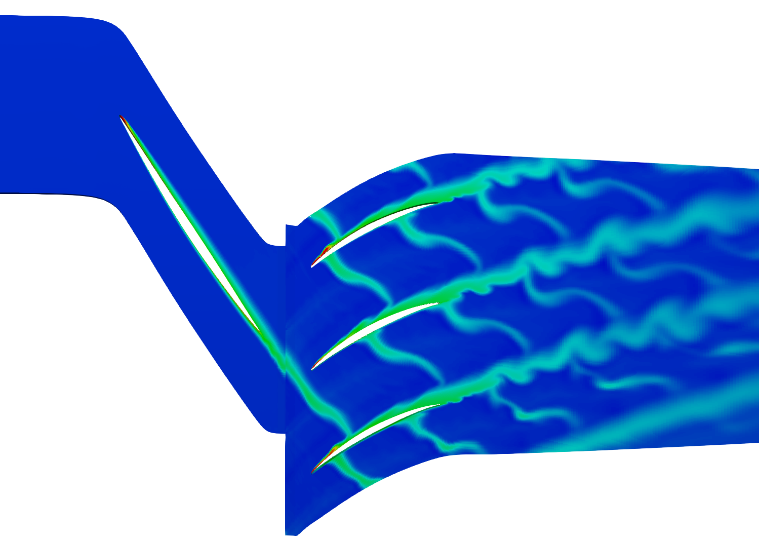
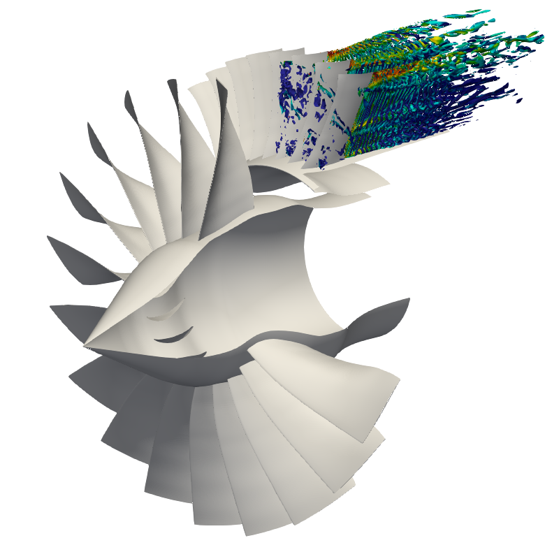
TURBOMACHINERY TONAL NOISE PREDICTION
Prediction of tonal noise of open rotors

- Harmonic Balance
- Non-reflective boundary conditions
- Non-reflective rotor/stator interface
- Ffowcs William & Hawking surface integration (convective formulation)
- Boundary conditions
- Number of harmonics needed
A periodic solution can be represented by an infinite series of harmonics
\[Q(t)=\sum_{n=-\infty}^{\infty}\hat{Q}_n e^{i\omega_n t}\]Truncating the series, we can get an approximation of the periodic solution
\[Q(t)\approx\sum_{n=-N_h}^{N_h}{\hat{Q}}_n e^{i\omega_n t}\]Nyquist sampling theorem:
A solution containing \(N_h\) harmonics is uniquely determined from its values at \(N_t=\left(2N_h+1\right)\) samples uniformly distributed over one period
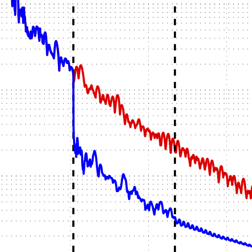
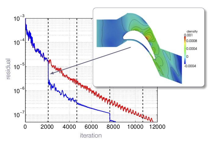
SOLVER ACCELERATION USING DMD
Assume that a problem has a true steady-state solution, could the global mode information provided by DMD be used to find the steady-state condition?
At steady state
\[Q^{(n+1)}=Q^{(n)}=Q\]and thus the linear relation
\[Q^{(n+1)}=BQ^{(n)}+b\]reduces to
\[(I-B)Q=b\]Introducing a correction \(\Delta Q\) that is obtained by subtracting sample \(Q^{(n+1)}\) from \(Q\), we get
\[(I-B)\Delta Q=\underbrace{(B-I)Q^{(n+1)}+b}_{\class{MyGreen}{Q^{(n+2)}-Q^{(n+1)}=D}}\]where the right hand side corresponds to the last vector in \(V_{n+1}\)
Introduce \(\Delta q\) defined by \(\Delta Q=U\Delta q\)
\[(I-B)\Delta Q=(I-B)U\Delta q={\class{MyGreen}{D}}\]Multiplying both sides with \(U^*\) from the left
\[{\class{MyRed}{U^*}}(I-{\class{MyRed}{B}}){\class{MyRed}{U}}\Delta q= \left\{ \class{MyBlue}{C}=\class{MyRed}{U^*BU},\ U^*U=I \right\}= (I-{\class{MyBlue}{C}})\Delta q = U^*{\class{MyGreen}{D}}\] \[\Rightarrow \Delta q = (I-{\class{MyBlue}{C}})^{-1}U^*{\class{MyGreen}{D}}\]From the definition of \(\Delta Q\) we get
\[Q=Q^{(n+1)}+\Delta Q=Q^{(n+1)}+U\Delta q\] \[Q=Q^{(n+1)}+U(I-{\class{MyBlue}{C}})^{-1}U^*{\class{MyGreen}{D}}\]where
\[{\class{MyBlue}{C}}=U^*V_{n+1}W\Sigma^{-1}\]Low-Mach-number (\(M<0.08\)) turbine cascade flow (2D)
STIRLING ENGINE
Stirling engine optimization


- Quasi-1D approach
- Modelling of heat transfer and flow losses
- Optimization
- Regenerator model
- Real gas effects
- Quasi-1D solver for simulating the flow in a Stirling engine developed
- Model validated against measured data
- Optimization framework setup and tested
COMPRESSOR BLADE OPTIMIZATION
Robust multi-objective optimization for compressor blade design
- Compressible RANS/URANS
- Multi-objective optimization
- Genetic algorithm
- Rotor tip-clearance
- Surge-margin prediction


ACOUSTIC RADIATION IN URBAN AREAS
Evaluation of noise canceling barriers for trains in urban areas

- Compressible DDES
- Ffowcs William & Hawking surface integration
- Spatial resolution
- Tonal noise source identification


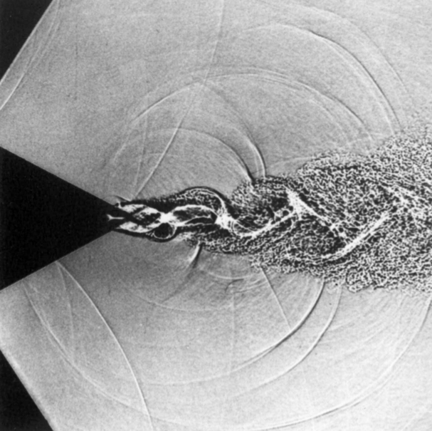
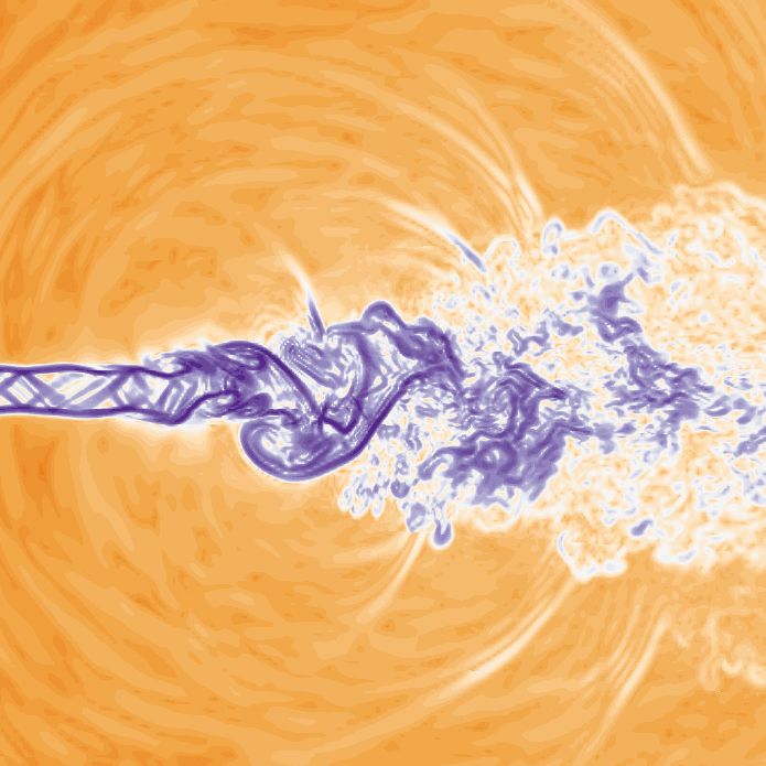
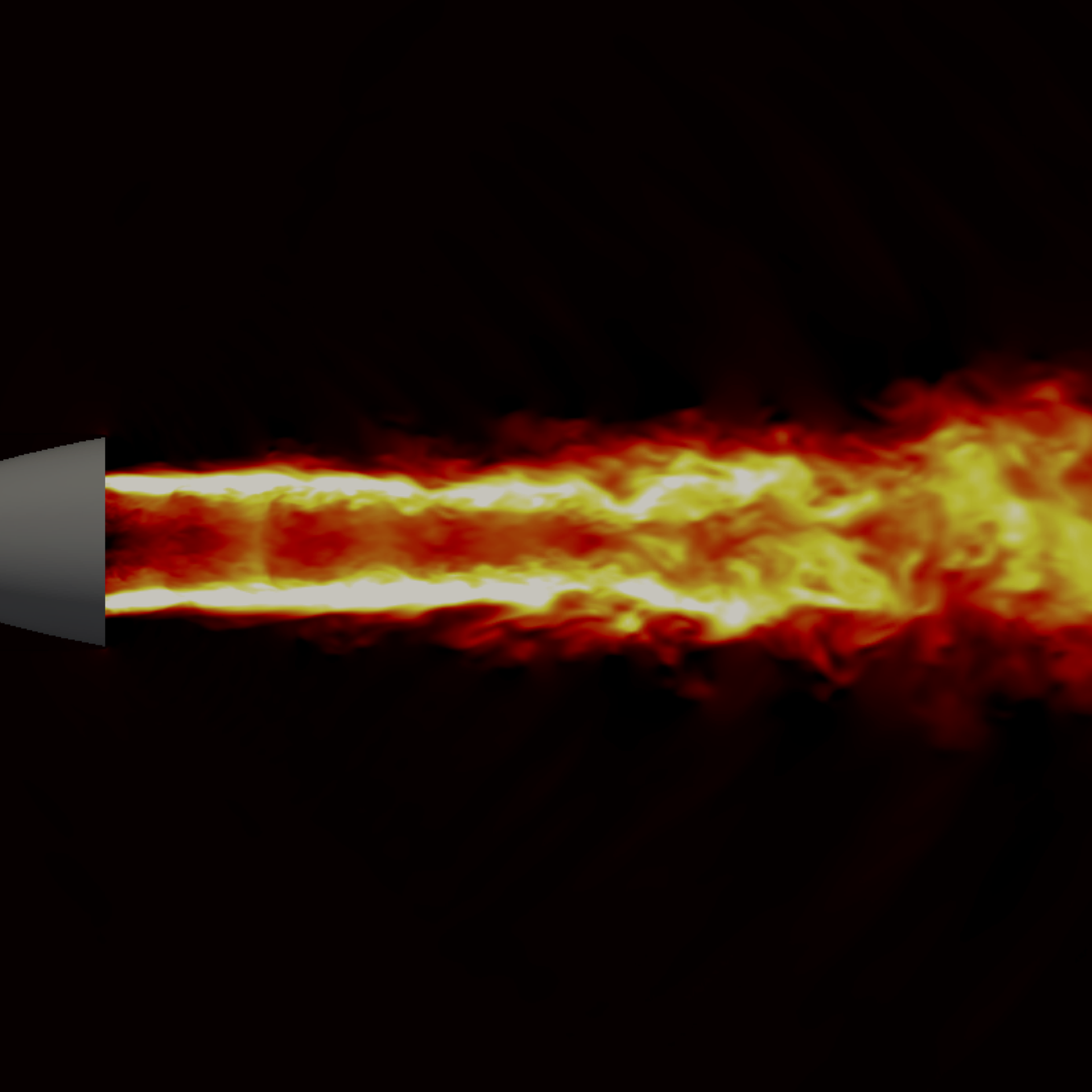
COMBUSTION INSTABILITIES
Prediction of combustion instabilities


- Compressible LES (Fluent)
- Combustion modelling
- Boundary conditions
- Prediction of sound generation and radiation
- Analyzing noise-generating flow mechanisms
- Low-noise design (optimization)
- geometric definition
- integrated acoustic liners
- Modular design of isolated components
- Detailed analysis of larger engine modules
- Engine module optimization
- Integrated design of engine components